Jacobian
Jacobian is Matrix in robotics which provides the relation between joint velocities ( ) & end-effector velocities ( ) of a robot manipulator.
If the joints of the robot move with certain velocities then we might want to know with what velocity the endeffector would move. Here is where Jacobian comes to our help. The relation between joint velocities and end-effector velocities is given as below,
where,
q is the column matrix representing the joint velocities. Size of the this matrix is nx1. 'n' is the number of joints of the robot.
x is the column matrix representing the end-effector velocities. Size of this matrix is mx1. 'm' is 3 for a planar robot and 6 for a spatial robot.
J is the Jacobian matrix which is a function of the current pose . Size of jacobian matrix is mxn.

Fig. 1 A spatial robot with n-joint/n-DOF
Let me write the above equation ( ) in expanded matrix form for a spatial robot for better understanding.

----------- ( )
*
Time to understand the Jacobian matrix.
Columns of the Jacobian matrix are associated with joints of the robot. Each column in the Jacobian matrix represents the effect on end-effector velocities due to variation in each joint velocity.
Which means, the first column represents the effect of joint1 velocity ( ) on end-effector velocities ( ), second column is associated with joint2 velocity ( ) and similarly nth column is effect of nth joint velocity ( ) on end-effector velocities .
Hence the number of columns in the Jacobian matrix is equal to the number of joints in the manipulator.
If we closely observe the x matrix, it has two parts.The first three elements of the end-effector velocity matrix are linear velocities [rate of change of position] and the last three elements are the angular velocites [rate of change of orientation] in (x,y,z) direction respectively.
Similarly, rows of the Jacobian matrix can also be split into two part. The first three rows are associated with linear velocities of end-effector and the last three rows are associated with the angular velocities of end-effector due to change in velocities of all the joints combined.
Hence we can call the upper part of the Jacobian matrix as Linear velocity Jacobian ( ) and the lower part as Angular velocity Jacobian ( ).

Now let's see how to derive a Jacobian matrix of robotic manipulator.
Methods to derive Jv and Jw are different. We will find them separately and later combine to get our final Jacobian matrix.
Finding Jv :
We all know from our elementary physics class that velocity is nothing but the first order derivative of position.Since Jv is related to linear velocities of the end-effector due to joint velocities, we can get the Jv by derivating the position functions for x, y and z of the end-effector w.r.t joint variables [ q1, q2, q3...........qn ] as shown below.

I guess by now a question would be running in your mind. Where from in this world we will get the functions for x, y and z.
I will give you a hint. The hint is Forward Kinematics.
Still confused, click here for the answer.
Yes you have got it right. The last column of the Transform matrix Tb-ee will provide us the functions for the position of end-effector.
We are half way through finding the Jacobian Matrix.
Lets find the second part.
Finding Jw :
Jw is related to the angular velocities of the end-effector. Again from our high school physic, we know that angular velocity ( ) is pseudo vector and is given by the product of axis of rotation ( ) and rate of rotation ( ) about the axis as shown in the below fig 2.

Fig. 2 A disk rotating about the axis with velocity radians/sec
is a unit vector representing the axis of rotation in 3D space. It is written in the below form,
Thus this unit vector can be represented as a 3x1 matrix as shown below,

Henceforth, angular velocity can be represented in matrix form as below
Angular velocity,

I have represented angular velocity in vector form to show you a similarity with Jacboian matrix in (*) equation above and make it simpler to find the matrix.
If we observe (*) equation, rate of rotation of all joints (joint velocities q1,q2,q3,....qn ) are already present in the [ ] matrix. So the only missing component to find the angular velocities of the end-effector is the axis of rotation information of each joint. This information, i.e., joint axes of all joints, is what jw matrix is all about.
Now there is a twist here in finding the joints axes . All joint axes in Jw are w.r.t base frame, not from the local frame.
Confused....??
Don't worry the below example will make things much clearer.
Look at the below fig 3. It is n link spatial manipulator. I have taken 3 joints i, j and k to explain you how to find the joint axes w.r.t base frame.
As the first job, I have attached frames to the links and lets say I have found the forward kinematics also.
The frames {i}, {j}, {k} are the local frames and {b} is the base frame to joints i, j and k respectively.

Fig. 3 A n-link Spatial manipulator with {b}, {i}, {j}, {k} focused
From fig 3 it is clear that joint i is rotating about z-axis of the local frame {i}, joint j about x-axis of local frame {j} and joint k about y-axis of local frame {k}. So the joint axes of joint i, j and k within their local frames are represented as below.

Axis of joint i w.r.t frame {i}

Axis of joint j w.r.t frame {j}

Axis of joint k w.r.t frame {k}
Finding the axis of the joint in the local frames looks easy right.
But we need the joint axis w.r.t to base frame {b} and finding this is not that straight forward. We have to pre-multiply the local joint axes with the rotation matrices respectively to get the joint axes w.r.t to base frame.
Axis of joint i w.r.t frame {b}
Axis of joint j w.r.t frame {b}
Axis of joint k w.r.t frame {b}
Looks tough right...?
But don't worry, we need not do the above multiplications to find the joint axes w.r.t frame {b}, there is a trick to find them easily.
These joint axes information is already present in one of the first three columns of the transform matrices Tbi, Tbj and Tbk (Tbi , Tbj and Tbk matrices would have been already derived while finding the forward kinematics). We just need to know the right column to look at. The right column information is provided by the axis of joint in local frame.
If the axis of rotation of joint in local frame is x, then first column of Tb? matrix is joint axis w.r.t base frame. Similarly, second column of Tb? for y-axis and third column for z-axis [Ignore the 0]
Note: To understand frame assignments and finding Transformations, go through Rigid Body Transformations
So we can get the joint axes from Tbi , Tbj and Tbk as shown below.


Isn't that simple.
Since we already know all the transform matrices from base to end-effector while finding the forward kinematics of our robot, therefore we have all joint axes w.r.t base frame information beforehand.
So all we need to do is group all these joint axes from joint-1 to joint-n [ ] to get the Jw matrix.
Finally....!! we have Jv and Jw. So we just have to stack them to get the complete Jacobian matrix.

Hurray..........!!!!!! we now know the in and out about the Jacobian matrix
A solved example to find the Jacobian matrix of a 6-DOF spatial manipulator is given below
But wait, the real question is still unanswered. How are we going to solve the inverse kinematics using Jacobian matrix.
So lets learn about the Jacobian Inversion Method.
Jacobian Inversion Method:
This method of inverse kinematics can be applied in two ways based on the type of joint actuators.
Method 1: For the robots with velocity controlled joint actuators.
Method 2: For the robots with position controlled joint actuators.
Before going to learn about the above two methods, lets re-frame the question and see what all values we know and what needs to be derived.
Q) Lets say we have n- link spatial robot as shown in below fig 4. The robot is at some random pose at this moment. Now the task is to move the end-effector of the robot to a given goal pose., Tg w.r.t base.

Fig. 4 A n-link Spatial manipulator
We can know joint position values [q1, q2, q3, ...., qn] of the current pose through the sensors (joint encoders) present at each joint. Hence we can get the Transformation matrix of the end-effector w.r.t base using FK. Lets call this transform matrix as Tc.
Since we have worked so hard to understand Jcobian matrix. By know we can derive Jacobian matrix. So we also know J matrix as the function of joint position values [q1, q2, q3, ...., qn].
Tg is given goal pose, so we know Tg as well.
Let me put all the known things in one frame.
1. Current Joint positions, q=[q1,q2,....qn]
2. Current end-effector position and orientation, Tc. From this Tc matrix we can get the Xc=[xc,yc,zc]
3. Goal position and orientation of end-effector Tg (or) Xg
4. Jacobian matrix [J] as function of current joint values.
Now lets see how to accomplish this task using Jacobian Inversion Method.
Method 1:
Since Jacobian gives a direct relation between end-effector velocities (X) and joint velocities (q) , the solution to inverse kinematics problem for a robot accepting velocity commands (radians/sec) is straight forward. All we need to do is to compute the end-effector velocities and Jacobian inverse. Finally find the joint velocities using below equation
Once we found the joint velocities, feed them to the joint actuators. In given time the end-effector will reach the desired goal pose. Once the goal pose is reached send 0 velocity commands to all the joint actuators to stop further movement of the robot.
That's all, our task of getting the end-effector to the desired pose is completed.
Lets write an algorithm for this method.
Step 1: Find AX.
AX=XG-Xc
Step 2: Convert AX into velocity X .
X.= P*AX
where p is simply a proportionality constant which decides the speed of the end-effector to reach the target pose.
Step 3: Using the current joint position values [q1,q2,q3................qn ], find the numerical value of Jacbian matrix.
Step 4: Find the pseudo inverse ( ) of the Jacobian matrix. (why pseudo inverse is discussed in the section Singularities).
Step 5: Compute q. using the below equation and feed the velocity commands to the joint actuators.
Step 6: Finally, track the pose of the end-effector and stop the joint actuator's movement once the goal pose is reached (i.e., AX = 0).
Method 2:
This method is applied to the robots whose joint actuators accepts position commands (radians). Which means we have to find new qn values (instead of q.) and feed them to joint actuators. Hence the Jacobian velocities equation cannot be used directly for this robots.
So we have to now make a relation between end-effector displacement and joint positions instead of their velocities. The same Jacobian equation can be used for displacement domain also but it only holds good for small displacements.
Whats "small displacement"..? There is no general recipe for that. It depends on the physical structure of the robots.
So we make AX a small displacement by multiplying it with some fraction value 'f' and using the above equation we get dq. This dq is added to the q to get the qne values. Now the qn values are given to joint actuators. Hence the end-effector move little closer to the goal pose.
Again AX is computed with the new Tc & given goal Tg and further qn values are computed in the same way. This is a iterative method. In each iteration end-effector gets closer-n-closer to the goal pose. Hence this is repeated until the goal pose is reached (i.e., AX=0).
Algorithm for this method
Step 1: Find AX .
AX=Xg-Xc
Step 2: Multiply AX with some fraction 'f' to make the displacement small
X.= delta*AX
where f is a fractional value and it is empirical.
Step 3: Using the current joint position values [q1,q2,q3................qn ], find the numerical value of Jacbian matrix.
Step 4: Find the pseudo inverse ( ) of the Jacobian matrix. (why pseudo inverse is discussed in the section Singularities).
Step 5: Compute dq using the below equation.
Step 6: Add dq to the current joint positions to get new joint position values
Step 7: Feed the new joint positions to the joint actuators and find the new Tc and Xc .
Step 8: Repeat 1 to 7 until AX =0.
Finally.....!!! we now know what is a Jacobian and how it is used to solve the inverse kinematics problem.
But we are not done yet. We only know the bright side of Jacobian method. Now lets talk about the dark side.
Problems with Jacobian Method:
Finding IK using this method involves matrix inversion. As we all know matrix inversion is not always easy and may not be possible in some cases. There are two such cases in this method where we would be facing trouble to find the inverse of J matrix.
1. When the Jacobian matrix is not a square matrix.
Can you guess for which robots the Jacobian matrix is not square..?
For the robots which has number of joints less than or greater than 6 but not exactly 6. i.e., when the robot is under-actuated or a redundant robot, the Jacobian matrix is not square.
2. When the robot is at Singularity.
There can be some pose of the robot where inverse may not be possible. This pose is know as singular configuration.
At singular configuration, Jacobian matrix loses its Rank, determinant of Jacobian becomes zero and inverse does not exits. Which physically means that the robot has lost a DOF. This usually happens when the end-effectoat the edges of the workspace i.e., when the robot is fully stretched.
However being in a singularity is not as bad as being very close to the singularity. When the robot is near to the singular configuration, it starts to behave abnormally when using this method.
This is because when the robot is approaching to singular configuration, the Jacobian inversion method will compute and produce lager joint velocities or delta q which is not acceptable. Asking for some finite movement in end-effector space can result in very very large, potentially infinite, movement in joint space which can have unpredictable results.
So while controlling our robot we have to make sure that our robot does not go into singular configuration and even more importantly we have to be careful not to approach singularities.
In Mathematics there is a solution to every problem. Luckily we have a common solution for both the problems mentioned above.
Solution to the Problems:
The solution is using Pseduo inverse ( J ) of the Jacobian matrix obtained by the Moore-Penrose matrix inversion instead of J-1.
1. This method uses Singular value decomposition to find the inverse of a non square matrix which is the solution to the first problem.
2. The inverse of a singular or non-invertible matrix is also possible with this method. And adiitionally the joint velocities or the delta q computed using pseudo inverse wont allow any additional movement towards the singularity but will allow any movement that doesn't get us any closer to the singularity. This solves our second problem of singularities.
Ta-Daa.....!! So we can happily use the jacobian invesion method to find the IK of the robot without any worries.
But I know you are still worried of one thing. That is how to find the Pseudo inverse of the Jacobian matrix. Isn't it..?
Well we are not going to discuss about the derivation of J+ from J matrix. Because, in practice we don't have to compute this by hand. Since the pseudo inverse is a very commonly used concept in linear algebra, almost any linear algebra library will have a function to compute it.
For example in python the pseudo inverse can b is found using below api in numpy lib.
Phew......!!! This ends our topic on Jacobian. Hoping you have understood everything about the Jacobian and enjoyed learning new things, I'll take leave. See you in the next topic.
J+=numpy.linalg.pinv(J,e)
Example 3:
In this example we find the Jacobian matrix of the 6-DOF robot shown in fig 12.

Fig. 5 6-DOF Spatial manipulator
As discussed in Jacobian Technique method, the no. of columns in Jacobian matrix depends on the no. of DOF of the robot. So no. of columns for our 6-DOF manipulator are 6.
Since this robot operates in the spatial workspace and it is a fully actuated robot, the no. of rows are also 6.
Therefore Jacobian for this manipulator is 6X6 square matrix.
The Jacobian matrix is derived using the Transformation matrix.

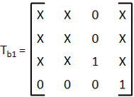
So lets start to find each Transformation matrices Tb1, Tb2,...... Tb-ee.
As we know to find the Transformations, the first step is frame assignment.

Fig. 6 Frames attached to our 6-DOF manipulator
As you have guessed, the next step is to write down the adjacent transformation matrices.


Now lets multiply these matrices to get the elements of the Jacobian matrix. (I will only show the required elements in the following matrices to build the Jacobian of our 6-DOF manipulator)


OMG that was a tedious job. I'm tired now. All the equations required for Jacobian matrix are already up there, kindly find the partial derivatives yourself and arrange all the elements to get the final J matrix. Thank you very much.
For any queries post your question in the comments section.